Using RMarkdown
Two weeks ago I presented in the weekly R Group Meeting of the Faculty of Life Sciences (University of Manchester) how to create RMarkdown files. These are files that combine calculation and plots from R with LaTeX-esque text objects. Why would you need to bother? Because it is a stunningly fast way to share your work and results from within R with your colleagues and supervisor. Furthermore, it sets an end to the time where I created a graph or calculated a p-value and lost track which R file contained the original commands. No more searching, you will have it all in place. And here is how it works (at least for Linux and MacOS, tell me if there are problems with Windows)
If you have the program RStudio and the R package knitr (just type in R install.packages(‘knitr’)) installed we we are ready to start.
-
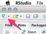
Open RStudio and click on the new file icon
-
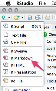
Select R Markdown to create a new Markdown
- RStudio will now open a template file. It already has a title some text and so called R chunks, which include R code as you would usually have in your R files.
- Add and change text and insert your R code (you can of course run the code in line or whole chunks). By the way, you find helpful information by clicking at the question mark icon in the top option bar of the source window (where you are currently entering your text). Click on Markdown Quick Reference to get an overview of useful commands. Click on Using R Markdown to get the full introduction from the RStudio website.
- If you are satisfied with the text and the data save the file in a new folder (I recommend a folder because the knitting process ends usually with a .Rmd, .md, and .html file, and maybe more files, but see below).
- Finally, click on Knit HTML to create your RMarkdown HTML file. The compiler will go through your text and your R chunks and create a Markdown file (.md) which it uses to return a HTML file.
Okay, let’s have a look how all these file may look like in the end. Copy and paste the following code in your source window and knit it to see what the result looks like.
The Gamma Distribution
========================================================
In _probability theory_ and statistics, the **gamma distribution** is a two-parameter family of continuous probability distributions.

The gamma distribution is described by a shape parameter $k$ and a scale parameter $\theta$. Its variance is $Var(X)=k*\theta^2$ and its mean is $E(X)=k*\theta$. The 'r 1+1'functions look like this in R:

```{r}
var_gamma <- function(k,t) return(k*(t^2))
mean_gamma <- function(k,t) return(k*t)

```

The next graph shows how the distribution changes with a chaging shape ($k$) value.

```{r, echo=FALSE, fig.width=10, fig.height=5}
plot(sort(rgamma(n=10000,shape=(K <- c(0.1,0.5,2,5,11)),scale=0.4)), type=‘l’, col=1, lwd=2, ylim=c(0,10), xlab=‘sorted values’, ylab=‘’)
for(k in K[-1]){
lines(sort(rgamma(n=10000,shape=k,scale=0.4)), lwd=2)
}
The resulting HTML file shout look like this:
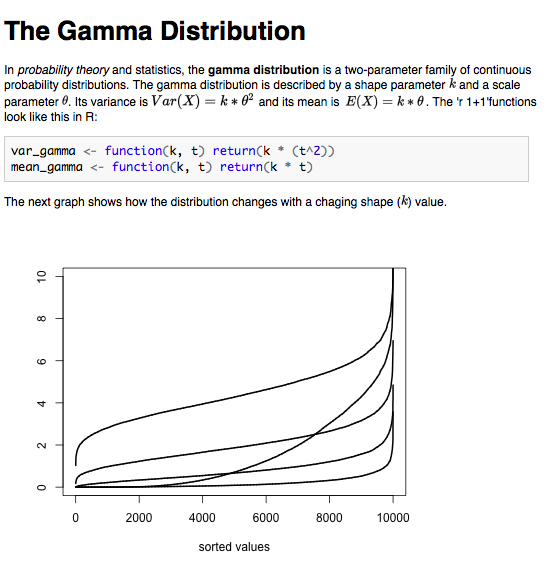
It is a minimal example of what you can do. We have there: a title, words in italic and bold letters, and even inline LaTeX code (it is flanked by dollar signs, find possible LaTeX symbol code here). I also included (obviously obsolete but for proof of principle) in line R code. It starts with r and ends with . In-between you can write whatever R code you want. You might want to calculate the sum or the mean of a data column or maybe a mean in combination with the standard deviation. You can use the following to do this:
    ```{r}
    DF <- data.frame(first=runif(10,0,1), second=runif(10,1,2))
    DF
    ```
    The mean value of the first experiment is $'r mean(DF$first)' \pm 'r sd(DF$first)'$.
Awesome, you get your results in line without writing any number down. This means also, that this is a very useful tool if you have report that you have to write repeatedly and only the numbers change. Just update the raw data and the report changes itself the next time you knit it. (Note, I combined LaTeX and R in-line code in the above example, yes it is possible).
You may find, that next to the introducing {r} there are sometimes further attributes like {r setup, echo=FALSE, results='hide'}. This line for example means the following:
- the chunk is called “setup”
- the code that you entered is not ‘echoed’ in the final document
- and all results are ‘hide’ in the final document
You might use this combination when you for example just want to load some function into your file that no-one else should see. The code is still evaluated. If you have code that you don’t want to evaluate (maybe it takes a long time to calculate or you don’t care for it at the moment) just add eval=FALSE. During the knitting process this chunk will not be evaluated.
Similarly, if you have a chunk that you only want to calculate once and want R to remember the results use cache=TRUE. This will save the results in a folder called ‘cache’. Every chunk with the argument cache=TRUE will be saved individually. As long as you don’t change the code in the chunk R will not calculate it again.
If you think that some of the graphs that you created during knitting would fit perfectly in another document, just go to the folder that you created for this document. You will find there a folder called figure, which contains all figures that R created during knitting as png files.
Finally, once you finished polishing your file and you want share it with your supervisor or colleague, it is enough to send the HTML file. All images are part of this HTML file due to the so called URI Scheme.
Now, enjoy having all your code, text and results stored in one place.